Sympy - Symbolic algebra in Python¶

J.R. Johansson (jrjohansson at gmail.com)

The latest version of this IPython notebook lecture is available at http://github.com/jrjohansson/scientific-python-lectures.

The other notebooks in this lecture series are indexed at http://jrjohansson.github.io.

%matplotlib inline
import matplotlib.pyplot as plt

Introduction¶

There are two notable Computer Algebra Systems (CAS) for Python:

SymPy - A python module that can be used in any Python program, or in an IPython session, that provides powerful CAS features.
Sage - Sage is a full-featured and very powerful CAS enviroment that aims to provide an open source system that competes with Mathematica and Maple. Sage is not a regular Python module, but rather a CAS environment that uses Python as its programming language.

Sage is in some aspects more powerful than SymPy, but both offer very comprehensive CAS functionality. The advantage of SymPy is that it is a regular Python module and integrates well with the IPython notebook.

In this lecture we will therefore look at how to use SymPy with IPython notebooks. If you are interested in an open source CAS environment I also recommend to read more about Sage.

To get started using SymPy in a Python program or notebook, import the module sympy:

from sympy import *

To get nice-looking \(\LaTeX\) formatted output run:

init_printing()

# or with older versions of sympy/ipython, load the IPython extension
#%load_ext sympy.interactive.ipythonprinting
# or
#%load_ext sympyprinting

Symbolic variables¶

In SymPy we need to create symbols for the variables we want to work with. We can create a new symbol using the Symbol class:

x = Symbol('x')

(pi + x)**2

# alternative way of defining symbols
a, b, c = symbols("a, b, c")

type(a)

sympy.core.symbol.Symbol

We can add assumptions to symbols when we create them:

x = Symbol('x', real=True)

x.is_imaginary

False

x = Symbol('x', positive=True)

x > 0

Complex numbers¶

The imaginary unit is denoted I in Sympy.

1+1*I

I**2

(x * I + 1)**2

Rational numbers¶

There are three different numerical types in SymPy: Real, Rational, Integer:

r1 = Rational(4,5)
r2 = Rational(5,4)

r1

r1+r2

r1/r2

Numerical evaluation¶

SymPy uses a library for artitrary precision as numerical backend, and has predefined SymPy expressions for a number of mathematical constants, such as: pi, e, oo for infinity.

To evaluate an expression numerically we can use the evalf function (or N). It takes an argument n which specifies the number of significant digits.

pi.evalf(n=50)

y = (x + pi)**2

N(y, 5) # same as evalf

When we numerically evaluate algebraic expressions we often want to substitute a symbol with a numerical value. In SymPy we do that using the subs function:

y.subs(x, 1.5)

N(y.subs(x, 1.5))

The subs function can of course also be used to substitute Symbols and expressions:

y.subs(x, a+pi)

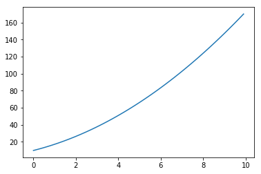
We can also combine numerical evolution of expressions with NumPy arrays:

import numpy

x_vec = numpy.arange(0, 10, 0.1)

y_vec = numpy.array([N(((x + pi)**2).subs(x, xx)) for xx in x_vec])

fig, ax = plt.subplots()
ax.plot(x_vec, y_vec);

However, this kind of numerical evolution can be very slow, and there is a much more efficient way to do it: Use the function lambdify to “compile” a Sympy expression into a function that is much more efficient to evaluate numerically:

f = lambdify([x], (x + pi)**2, 'numpy')  # the first argument is a list of variables that
                                         # f will be a function of: in this case only x -> f(x)

y_vec = f(x_vec)  # now we can directly pass a numpy array and f(x) is efficiently evaluated

The speedup when using “lambdified” functions instead of direct numerical evaluation can be significant, often several orders of magnitude. Even in this simple example we get a significant speed up:

%%timeit

y_vec = numpy.array([N(((x + pi)**2).subs(x, xx)) for xx in x_vec])

10 loops, best of 3: 20 ms per loop

%%timeit

y_vec = f(x_vec)

The slowest run took 16.37 times longer than the fastest. This could mean that an intermediate result is being cached.
100000 loops, best of 3: 3 µs per loop

Algebraic manipulations¶

One of the main uses of an CAS is to perform algebraic manipulations of expressions. For example, we might want to expand a product, factor an expression, or simply an expression. The functions for doing these basic operations in SymPy are demonstrated in this section.

Expand and factor¶

The first steps in an algebraic manipulation

(x+1)*(x+2)*(x+3)

expand((x+1)*(x+2)*(x+3))

The expand function takes a number of keywords arguments which we can tell the functions what kind of expansions we want to have performed. For example, to expand trigonometric expressions, use the trig=True keyword argument:

sin(a+b)

expand(sin(a+b), trig=True)

See help(expand) for a detailed explanation of the various types of expansions the expand functions can perform.

The opposite a product expansion is of course factoring. The factor an expression in SymPy use the factor function:

factor(x**3 + 6 * x**2 + 11*x + 6)

Simplify¶

The simplify tries to simplify an expression into a nice looking expression, using various techniques. More specific alternatives to the simplify functions also exists: trigsimp, powsimp, logcombine, etc.

The basic usages of these functions are as follows:

# simplify expands a product
simplify((x+1)*(x+2)*(x+3))

# simplify uses trigonometric identities
simplify(sin(a)**2 + cos(a)**2)

simplify(cos(x)/sin(x))

apart and together¶

To manipulate symbolic expressions of fractions, we can use the apart and together functions:

f1 = 1/((a+1)*(a+2))

f1

apart(f1)

f2 = 1/(a+2) + 1/(a+3)

f2

together(f2)

Simplify usually combines fractions but does not factor:

simplify(f2)

Calculus¶

In addition to algebraic manipulations, the other main use of CAS is to do calculus, like derivatives and integrals of algebraic expressions.

Differentiation¶

Differentiation is usually simple. Use the diff function. The first argument is the expression to take the derivative of, and the second argument is the symbol by which to take the derivative:

diff(y**2, x)

For higher order derivatives we can do:

diff(y**2, x, x)

diff(y**2, x, 2) # same as above

To calculate the derivative of a multivariate expression, we can do:

x, y, z = symbols("x,y,z")

f = sin(x*y) + cos(y*z)

\(\frac{d^3f}{dxdy^2}\)

diff(f, x, 1, y, 2)

Integration¶

Integration is done in a similar fashion:

integrate(f, x)

\[\begin{split}x \cos{\left (y z \right )} + \begin{cases} 0 & \text{for}\: y = 0 \\- \frac{1}{y} \cos{\left (x y \right )} & \text{otherwise} \end{cases}\end{split}\]

By providing limits for the integration variable we can evaluate definite integrals:

integrate(f, (x, -1, 1))

and also improper integrals

integrate(exp(-x**2), (x, -oo, oo))

Remember, oo is the SymPy notation for inifinity.

Sums and products¶

We can evaluate sums and products using the functions: ‘Sum’

n = Symbol("n")

Sum(1/n**2, (n, 1, 10))

Sum(1/n**2, (n,1, 10)).evalf()

Sum(1/n**2, (n, 1, oo)).evalf()

Products work much the same way:

Product(n, (n, 1, 10)) # 10!

Limits¶

Limits can be evaluated using the limit function. For example,

limit(sin(x)/x, x, 0)

We can use ‘limit’ to check the result of derivation using the diff function:

diff(f, x)

\(\displaystyle \frac{\mathrm{d}f(x,y)}{\mathrm{d}x} = \frac{f(x+h,y)-f(x,y)}{h}\)

h = Symbol("h")

limit((f.subs(x, x+h) - f)/h, h, 0)

OK!

We can change the direction from which we approach the limiting point using the dir keywork argument:

limit(1/x, x, 0, dir="+")

limit(1/x, x, 0, dir="-")

Series¶

Series expansion is also one of the most useful features of a CAS. In SymPy we can perform a series expansion of an expression using the series function:

series(exp(x), x)

By default it expands the expression around \(x=0\), but we can expand around any value of \(x\) by explicitly include a value in the function call:

series(exp(x), x, 1)

And we can explicitly define to which order the series expansion should be carried out:

series(exp(x), x, 1, 10)

The series expansion includes the order of the approximation, which is very useful for keeping track of the order of validity when we do calculations with series expansions of different order:

s1 = cos(x).series(x, 0, 5)
s1

s2 = sin(x).series(x, 0, 2)
s2

expand(s1 * s2)

If we want to get rid of the order information we can use the removeO method:

expand(s1.removeO() * s2.removeO())

But note that this is not the correct expansion of \(\cos(x)\sin(x)\) to \(5\)th order:

(cos(x)*sin(x)).series(x, 0, 6)

Linear algebra¶

Matrices¶

Matrices are defined using the Matrix class:

m11, m12, m21, m22 = symbols("m11, m12, m21, m22")
b1, b2 = symbols("b1, b2")

A = Matrix([[m11, m12],[m21, m22]])
A

\[\begin{split}\left[\begin{matrix}m_{11} & m_{12}\\m_{21} & m_{22}\end{matrix}\right]\end{split}\]

b = Matrix([[b1], [b2]])
b

\[\begin{split}\left[\begin{matrix}b_{1}\\b_{2}\end{matrix}\right]\end{split}\]

With Matrix class instances we can do the usual matrix algebra operations:

A**2

\[\begin{split}\left[\begin{matrix}m_{11}^{2} + m_{12} m_{21} & m_{11} m_{12} + m_{12} m_{22}\\m_{11} m_{21} + m_{21} m_{22} & m_{12} m_{21} + m_{22}^{2}\end{matrix}\right]\end{split}\]

A * b

\[\begin{split}\left[\begin{matrix}b_{1} m_{11} + b_{2} m_{12}\\b_{1} m_{21} + b_{2} m_{22}\end{matrix}\right]\end{split}\]

And calculate determinants and inverses, and the like:

A.det()

A.inv()

\[\begin{split}\left[\begin{matrix}\frac{m_{22}}{m_{11} m_{22} - m_{12} m_{21}} & - \frac{m_{12}}{m_{11} m_{22} - m_{12} m_{21}}\\- \frac{m_{21}}{m_{11} m_{22} - m_{12} m_{21}} & \frac{m_{11}}{m_{11} m_{22} - m_{12} m_{21}}\end{matrix}\right]\end{split}\]

Solving equations¶

For solving equations and systems of equations we can use the solve function:

solve(x**2 - 1, x)

solve(x**4 - x**2 - 1, x)

System of equations:

solve([x + y - 1, x - y - 1], [x,y])

In terms of other symbolic expressions:

solve([x + y - a, x - y - c], [x,y])

Versions¶

%reload_ext version_information

%version_information numpy, matplotlib, sympy

ImportErrorTraceback (most recent call last)
<ipython-input-90-00c7a10bc885> in <module>()
----> 1 get_ipython().magic(u'reload_ext version_information')
      2 
      3 get_ipython().magic(u'version_information numpy, matplotlib, sympy')

/usr/local/lib/python2.7/dist-packages/IPython/core/interactiveshell.pyc in magic(self, arg_s)
   2158         magic_name, _, magic_arg_s = arg_s.partition(' ')
   2159         magic_name = magic_name.lstrip(prefilter.ESC_MAGIC)
-> 2160         return self.run_line_magic(magic_name, magic_arg_s)
   2161 
   2162     #-------------------------------------------------------------------------

/usr/local/lib/python2.7/dist-packages/IPython/core/interactiveshell.pyc in run_line_magic(self, magic_name, line)
   2079                 kwargs['local_ns'] = sys._getframe(stack_depth).f_locals
   2080             with self.builtin_trap:
-> 2081                 result = fn(*args,**kwargs)
   2082             return result
   2083 

</usr/local/lib/python2.7/dist-packages/decorator.pyc:decorator-gen-65> in reload_ext(self, module_str)

/usr/local/lib/python2.7/dist-packages/IPython/core/magic.pyc in <lambda>(f, *a, **k)
    186     # but it's overkill for just that one bit of state.
    187     def magic_deco(arg):
--> 188         call = lambda f, *a, **k: f(*a, **k)
    189 
    190         if callable(arg):

/usr/local/lib/python2.7/dist-packages/IPython/core/magics/extension.pyc in reload_ext(self, module_str)
     65         if not module_str:
     66             raise UsageError('Missing module name.')
---> 67         self.shell.extension_manager.reload_extension(module_str)

/usr/local/lib/python2.7/dist-packages/IPython/core/extensions.pyc in reload_extension(self, module_str)
    126                 self.loaded.add(module_str)
    127         else:
--> 128             self.load_extension(module_str)
    129 
    130     def _call_load_ipython_extension(self, mod):

/usr/local/lib/python2.7/dist-packages/IPython/core/extensions.pyc in load_extension(self, module_str)
     81             if module_str not in sys.modules:
     82                 with prepended_to_syspath(self.ipython_extension_dir):
---> 83                     __import__(module_str)
     84             mod = sys.modules[module_str]
     85             if self._call_load_ipython_extension(mod):

ImportError: No module named version_information

---------------------------------------------------------------------------
NOTE: If your import is failing due to a missing package, you can
manually install dependencies using either !pip or !apt.

To view examples of installing some common dependencies, click the
"Open Examples" button below.
---------------------------------------------------------------------------

Scientific Python QuickStart